GIS Internship - GIS Portfolio

GIS Portfolio link: ftp://ftp.students.uwf.edu/web/Greg_Leenig_GIS_Portfolio.pdf

This is my GIS portfolio that I created for my GIS Internship course. It took a while to make, but I think the quality is pretty good. It includes an about me, resume, map samples, and transcripts. The portfolio is worthwhile to make because you have evidence of what kind of work you have done in the past. I will use this when looking for GIS positions.

ArcMap Ground Truthing LULC

Lab Objectives:

By the end of this lab, students should be able to:

• Construct an unbiased sampling system
• Locate and identify features using Google Maps street view
• Calculate the accuracy of a Land Use / Land Cover classification map 

This lab focused on establishing accuracy in land classification using ground truthing. Adding the LULC map from the previous lab in ArcMap, I randomly marked 30 points around the map. Then, using Google Maps and Streetview, I judged whether the feature at each point actually corresponded with the land classification. If it did, I indicated that the point was accurate. If it did not, I indicated the point was inaccurate. After doing this for all 30 points, I calculated the overall accuracy of sample points to land classification. I changed the symbology of the points to green for accurate points and red for inaccurate points. This resulted in an updated LULC map, seen below.

The map above still shows the overall land classifications and LULC codes for Pascagoula, Mississippi, but it is also updated to show the ground truthing and point accuracy.

ArcMap LULC Land Classification

Lab Objectives:

By the end of this lab, students should be able to:

• Apply recognition elements to Land Use Land Cover (LULC) classification
• Identify various features using aerial photography
• Construct a land use / land cover map 

This lab involved identifying features from aerial photography and classifying features into land use classes. The study area is Pascagoula, Mississippi. To classify features, I added a polygon shapefile to ArcMap, which was layed over a TIF true color image of Pascagoula. Using an edit session, I was able to make many polygons of features and then classify those polygons. The polygons were color-coded corresponding to class, and transparency was made so that features could still be seen. These polygons were classified by LULC codes and code descriptions. Polygons were made at a large scale at first (such as classifying the bay, wetlands, and residential areas), but got a little more detailed further into the process (such as classifying commercial, industrial, lakes, etc.). Classifications were made at least to level 2, sometimes level 3.

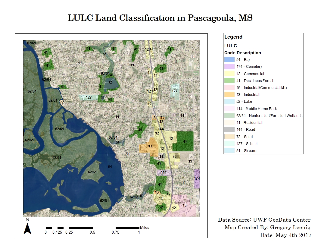
The map above classifies various land features in the study area. The numbers in the legend are the LULC codes.

ERDAS Supervised Classification

Lab Objectives:

By the end of this lab, students should be able to:

• Create spectral signatures and AOI features 
• Produce classified images from satellite data 
• Recognize and eliminate spectral confusion between spectral signatures

This lab involved collecting/creating spectral signatures and classifying them. This is done under supervision (by the creator/user) instead of the computer program. Creating spectral signatures can be done by manually drawing polygons to classify the area of interest (AOI) after an AOI layer is established, and also by growing "seeds" (using spectral euclidean distance and neighborhood). The user can evaluate signatures and appropriate bands by using histogram plots and signature mean plots. These can be used to mitigate spectral confusion between classes.

The image of interest is classified by having the signature file undergo the supervised classification process. Optionally, the user can also create at the same time a distance file image, which shows possible error in the classified image. After this, the user can merge certain classes of the new supervised image if the user wishes. After the classes are merged (or recoded), class names can be established in the recoded image and area of each class can be calculated. The supervised classification process was done during this lab to create land classification of Germantown, Maryland.

The map above shows land classification in the area, such as agriculture, urban, forest, grass, etc.

ArcMap and ERDAS Unsupervised Classification

Lab Objectives:

By the end of this lab, students should be able to:

• Perform an unsupervised classification in both ArcMap and ERDAS 
• Accurately classify images of different spatial and spectral resolutions 
• Manually reclassify and recode images to simplify the data 

In this lab, I performed unsupervised classification, as well as reclassify and recode these classes. First, using ArcMap, I created a classified image by using the Iso Cluster tool and Maximum Likelihood Classification tool on a raster image. I then examined the new image and properly reclassified the classes and used an appropriate color to represent each class.

In ERDAS Imagine, I used the ISODATA (Iterative Self-Organizing Data Analysis Technique) algorithm to perform an unsupervised classification on a raster image of UWF campus. Once the output image was created and added to ERDAS, I reclassified all 50 classes to proper classes, such as grass, trees, shadows, and buildings and roads. To refine the reclassification step, I used methods such as swipe, flicker, blend, and highlight. I then merged these classes by recoding them into five distinct classes. Using these five classes, I calculated the percentage area of permeable and impermeable surfaces.

The map above represents the land classification of UWF campus.

Spatial Enhancement

Lab Objectives:

By the end of this lab, students should be able to:
1. Download and import satellite imagery
2. Perform spatial enhancements in ArcMap and ERDAS
3. Utilize the Fourier Transformation function

The beginning of this lab (Exercise 1) focused on the process of acquiring satellite data. USGS Earth Explorer was used to identify correct imagery. The imagery could be downloaded and extracted, and then the imagery could be converted to the correct format and reprojected to the correct coordinate system. If needed, preprocessing (like image subsetting and image enhancement) could be conducted as well.

In ERDAS, Exercise 2 focused on importing data, changing the format from TIFF to IMG (using the batch option for multiple files), and creating a multispectral image from multiple panchromatic files using the layer stack tool.

Exercise 3 focused on spatial/image enhancements. In ERDAS, basic low and high pass filters were used to improve images (using the convolution tool). In ArcMap other filters were used, specifically focal statistics using mean and range to improve images.

Exercise 4 focused on image enhancements in ERDAS. An image of the Pensacola area was used, and there was a lot of striping in the image. Fourier transformation, using the wedge tool and the low pass tool, was utilized on this striped image. This removed much of the striping in the image. The convolution filter, using the 3x3 Sharpen Kernel, was used to sharpen the image. At the end of Exercise 4, I used Fourier transformation and the convolution filter again to remove even more of the striping and increase the sharpness. I used this final image to create a map.

Remote Sensing - ERDAS Imagine and Digital Data

Lab Objectives:

• Utilize tools and functions of ERDAS Imagine
• Interpret Layer Info of digital data in ERDAS Imagine
• Distinguish between the four types of resolution in ERDAS Imagine
• Interpret and analyze thematic rasters in ERDAS Imagine

This lab involved using ERDAS Imagine to obtain information about images, examining various types of resolution in images, examining how these resolutions were relevant to digital data being captured, stored, and displayed, and learning how to interpret and analyze a thematic (soil) raster.

In the first exercise, metadata was used to examine layer properties of specific "layers", or bands. Layer properties included file info, layer info, statistics info, map info, and projection info. Data type (bit), under layer info, represents radiometric resolution. Pixel size, under map info, represents spatial resolution.

The second exercise focused on four types of resolution: radiometric, spatial, spectral, and temporal. Spatial resolution is determined by the pixel size of the image. The smaller the pixel size, the higher the spatial resolution. However, higher resolution also means larger file sizes. Spatial resolution is the most common type of resolution: it is often referred to just as "resolution". Spatial resolution was compared among four identical images, however the spatial resolution of the images varied from high to low, showing different levels of detail.

Radiometric resolution is described as the detail of an image based on the level of contrast between objects. The radiometric resolution of an imaging system describes its ability to discriminate very slight differences in energy. The finer the radiometric resolution of a sensor, the more sensitive it is to detecting small differences in reflected or emitted energy. Max digital number (DN), under statistics info, represents the highest brightness value for all the pixels in the image. Max DN corresponds to data type, or bit. The higher the DN (max 255), the higher the bit (max 8-bit). Four images with varying radiometric resolutions (high to low) were compared. The last image had the lowest radiometric resolution, showing only black and white contrast. However, the first image had the highest resolution, showing varying contrast: white, black, but also varying levels of gray.

Spectral resolution is how well an image can be used to distinguish between different wavelengths, or bands. Two things contribute to the spectral resolution of an image: the number of bands and the wavelengths that they cover. The more bands an image has, and the narrower the bandwidths, the higher the spectral resolution. Two images were compared. One image was multispectral, having multiple bands, while the other had only one band. Thus, the multispectral image had higher spectral resolution.

Temporal resolution is how frequently an image of the same area can be taken. Temporal resolution usually deals with the orbit of a satellite. Landsat 7, for instance, passes over the same area every 16 days. The Landsat images then have a temporal resolution of 16 days.

The third exercise involved computing area and percent area coverage of different soil types. Also, soil types with high susceptibility to erosion were defined, displayed, and highlighted. An image of the final result was then saved.