Spatial Enhancement

Lab Objectives:

By the end of this lab, students should be able to:
1. Download and import satellite imagery
2. Perform spatial enhancements in ArcMap and ERDAS
3. Utilize the Fourier Transformation function

The beginning of this lab (Exercise 1) focused on the process of acquiring satellite data. USGS Earth Explorer was used to identify correct imagery. The imagery could be downloaded and extracted, and then the imagery could be converted to the correct format and reprojected to the correct coordinate system. If needed, preprocessing (like image subsetting and image enhancement) could be conducted as well.

In ERDAS, Exercise 2 focused on importing data, changing the format from TIFF to IMG (using the batch option for multiple files), and creating a multispectral image from multiple panchromatic files using the layer stack tool.

Exercise 3 focused on spatial/image enhancements. In ERDAS, basic low and high pass filters were used to improve images (using the convolution tool). In ArcMap other filters were used, specifically focal statistics using mean and range to improve images.

Exercise 4 focused on image enhancements in ERDAS. An image of the Pensacola area was used, and there was a lot of striping in the image. Fourier transformation, using the wedge tool and the low pass tool, was utilized on this striped image. This removed much of the striping in the image. The convolution filter, using the 3x3 Sharpen Kernel, was used to sharpen the image. At the end of Exercise 4, I used Fourier transformation and the convolution filter again to remove even more of the striping and increase the sharpness. I used this final image to create a map.

Remote Sensing - ERDAS Imagine and Digital Data

Lab Objectives:

• Utilize tools and functions of ERDAS Imagine
• Interpret Layer Info of digital data in ERDAS Imagine
• Distinguish between the four types of resolution in ERDAS Imagine
• Interpret and analyze thematic rasters in ERDAS Imagine

This lab involved using ERDAS Imagine to obtain information about images, examining various types of resolution in images, examining how these resolutions were relevant to digital data being captured, stored, and displayed, and learning how to interpret and analyze a thematic (soil) raster.

In the first exercise, metadata was used to examine layer properties of specific "layers", or bands. Layer properties included file info, layer info, statistics info, map info, and projection info. Data type (bit), under layer info, represents radiometric resolution. Pixel size, under map info, represents spatial resolution.

The second exercise focused on four types of resolution: radiometric, spatial, spectral, and temporal. Spatial resolution is determined by the pixel size of the image. The smaller the pixel size, the higher the spatial resolution. However, higher resolution also means larger file sizes. Spatial resolution is the most common type of resolution: it is often referred to just as "resolution". Spatial resolution was compared among four identical images, however the spatial resolution of the images varied from high to low, showing different levels of detail.

Radiometric resolution is described as the detail of an image based on the level of contrast between objects. The radiometric resolution of an imaging system describes its ability to discriminate very slight differences in energy. The finer the radiometric resolution of a sensor, the more sensitive it is to detecting small differences in reflected or emitted energy. Max digital number (DN), under statistics info, represents the highest brightness value for all the pixels in the image. Max DN corresponds to data type, or bit. The higher the DN (max 255), the higher the bit (max 8-bit). Four images with varying radiometric resolutions (high to low) were compared. The last image had the lowest radiometric resolution, showing only black and white contrast. However, the first image had the highest resolution, showing varying contrast: white, black, but also varying levels of gray.

Spectral resolution is how well an image can be used to distinguish between different wavelengths, or bands. Two things contribute to the spectral resolution of an image: the number of bands and the wavelengths that they cover. The more bands an image has, and the narrower the bandwidths, the higher the spectral resolution. Two images were compared. One image was multispectral, having multiple bands, while the other had only one band. Thus, the multispectral image had higher spectral resolution.

Temporal resolution is how frequently an image of the same area can be taken. Temporal resolution usually deals with the orbit of a satellite. Landsat 7, for instance, passes over the same area every 16 days. The Landsat images then have a temporal resolution of 16 days.

The third exercise involved computing area and percent area coverage of different soil types. Also, soil types with high susceptibility to erosion were defined, displayed, and highlighted. An image of the final result was then saved.

Remote Sensing - Intro to ERDAS Imagine

Lab Objectives:

• Calculate wavelength, frequency, and energy of EMR
• Locate and use basic tools in ERDAS Imagine
• Learn about and use the Viewer to view data in ERDAS Imagine
• Subset data in ERDAS Imagine as a preprocessing step for making a map in ArcGIS

ERDAS is a computer program specialized for remote sensing data. This program is new to me, but the lab this week was a good introduction to ERDAS. The lab began with the first exercise, giving a quality introduction to important remote sensing concepts, such as EMR, wavelength, frequency, light spectrum, etc.

The second exercise really focused on the ERDAS program. I was introduced to important introductory information, such as the overall layout/interface of the program, adding data to different specifications, navigating controls like zoom and pan, and using multiple viewing windows to work with more than one image at a time. Towards the end of exercise 2, the exercise showed different types of imaging techniques and combinations of bands, such as False Natural Color and False Color IR. Different bands can reveal or "highlight" certain objects and/or land cover.

The third and last exercise revolved around data preparation with ERDAS and map-making with that data. A remotely-sensed raster image was used, and it showed classified land areas, such as bare ground, cloud, water, riparian, and vegetation classed by aspect. Each class was made up of a combination of red, green, and blue bands. Using this preliminary image, a subset image was taken of a small area using ERDAS. This subset image was added to a viewing window in ERDAS, and an area column was added to the attribute table of the subset image. Area (in hectares) was calculated for each classification type. After editing this attribute table, the image file needed to be saved again.
This saved image was then added to ArcMap, and the classes were reclassified. A map was then created to display the classes in the study area.

Overall, this lab was a little time consuming because I was learning a new GIS program. However, it was enjoyable to apply remote sensing techniques/images to GIS and see "real world" applications.

Remote Sensing - Visual Interpretation of Aerial Photography

Lab Objectives:

• Interpret tone and texture of aerial photographs
• Identify land features in an aerial photograph based on several visual attributes
• Compare similar land features in true color and false color IR photographs

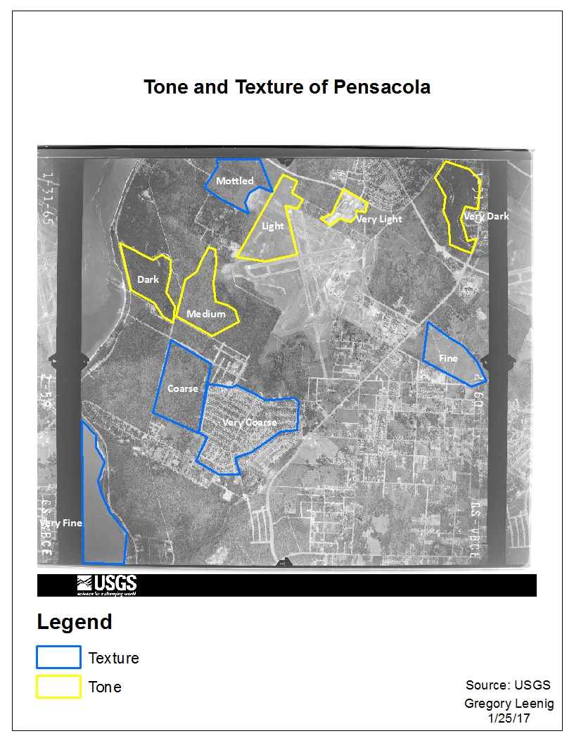
This lab focused on visual interpretation of aerial photography, such as tone and texture gradients, identifying land features, and comparing land features in true color and false color infrared photographs. 

        

In the first exercise I identified areas based on tone, ranging from very dark to very light. I also identified areas based on texture (or roughness), ranging from very coarse to very fine. 

In the second exercise, I identified land features based on patterns, shadows, shape and size, and associations. 

For the third exercise I compared two photographs (one true color and one false color infrared) of the North Pensacola area. I compared land features, such as trees, rivers, buildings, marsh, and observed color differences in these features between the photographs. 

I found it a little difficult to classify tone and texture, because sometimes there were subtle differences between the classes. However, I found it interesting that there are specific ways to identify and classify features in aerial photographs. Also, comparing photographs and features based on true color and false color is a new and interesting area of GIS for me.